Basics of RNN and LSTM for non data scientists

(But you need to know Maths)

In this article, I give a simple mathematical exposition of RNN (Recurrent Neural Network) and LSTM (Long Short Term Memory) models- if you are comfortable with matrix multiplication, you will understand RNN and LSTM from this article, even if you don't have prior experience in data science. While there are great resources on this topic (e.g. this one), most articles on these topics are written by data scientists who assume some data science concepts or notations, which an outside struggles with. Since I learnt it as a non professional data scientist, I might be able to better explain it to you if you are not a data scientist.

At Simpl, we use sequence models heavily and I had a chance to sit with Yash and Nikita, with whose help I was able to understand the models, to a level that makes me feel a bit educated.

Some preliminaries and notations

1. Our anchor problem

While RNNs can be used to solve many problems related to sequential data, we will use the anchor problem of translating one language sentence to another. We have a lot of translations available and we want to use them to train language translation model.

2. Word embedding and softmax

Our models don't directly operate on string representations of the words of the language. Rather, they operate on vector representation of those words. A "word embedding" converts words to a row matrix of floating point numbers, and a "softmax" function converts a vector to a word. Understanding word embedding or softmax is outside the scope of this article. Input vectors for a single source language sentence would be denoted by $x_1, x_2, \dots x_t\dots $, and output vectors for a single destination language sentence would be denoted by $y_1, y_2, \dots y_t, \dots$. Note that each of $x_i$ and $y_i$ is a row vector.

In the article below, assume that the each $x_t$ is a $n \times 1$ vector and each $y_t$ is an $o \times 1$ vector.

3. Sigmoid function

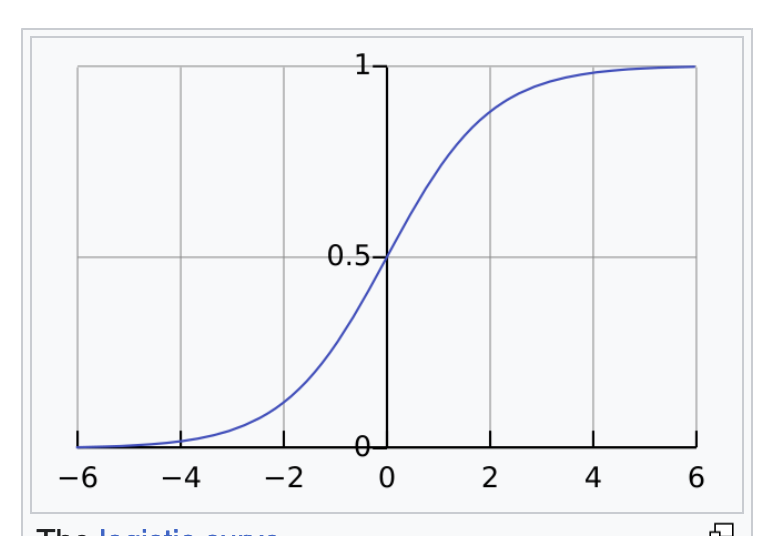
There is a function called sigmoid function, denoted by $\sigma$ which converts a real number to a number between 0 and 1: $$\sigma(x) = \dfrac{1}{1+e^{-x}}$$ This is what the sigmoid function looks like

We also define this function over matrices by applying sigmod to each element. So, $$\sigma\left( \begin{bmatrix} 5 & 6\\ 7 & 8\\ 9 & 10\\ 11 & 12 \end{bmatrix} \right) = \begin{bmatrix} \sigma(5) & \sigma(6)\\ \sigma(7) & \sigma(8)\\ \sigma(9) & \sigma(10)\\ \sigma(11) & \sigma(12) \end{bmatrix} $$

4. Hyperbolic tangent function

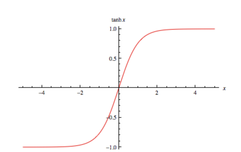
$$\tanh(x) = \dfrac{e^x - e^{-x}}{e^x + e^{-x}}$$ This is the graph of $\tanh(x)$

Hyperbolic tangent function is also defined over a matrix - we apply it to each element. Thus: $$\tanh\left( \begin{bmatrix} 5 & 6\\ 7 & 8\\ 9 & 10\\ 11 & 12 \end{bmatrix} \right) = \begin{bmatrix} \tanh(5) & \tanh(6)\\ \tanh(7) & \tanh(8)\\ \tanh(9) & \tanh(10)\\ \tanh(11) & \tanh(12) \end{bmatrix} $$

5. Use of $\sigma(x)$ and $\tanh(x)$ in deep learning

This is the way I look at it:
In any deep learning model, input $x$ (think of $x$ like a column vector) could have been transfered to output $y$ by successive matrix multiplications:

Here $A_1, A_2, A_3, \dots$ are the matrices that your model learns - their values are set as a part of training. But since $A_3(A_2(A_1))x = (A_3 \times A_2 \times A_1)x$, there is no additional expressive power because of so many matrices - they can all be compressed into just one matrix $B = A_3 \times A_2 \times A_1$.

When you introduce non linearity -

then the model becomes more expressive since we cannot collapse all these operations to single operation. This non linearity allows a preferential flow of some values compared to to other to the next step, and that is what gives neural network its power.

6. dot(.) and odot($\odot$) notation

In this article, dot(.) denotes matrix multiplication: $$ \begin{bmatrix} 1 & 2\\ 3 & 4\\ \end{bmatrix} . \begin{bmatrix} 5 & 6\\ 7 & 8\\ \end{bmatrix} = \begin{bmatrix} 19 & 22\\ 43 & 50\\ \end{bmatrix} $$

odot($\odot$) denotes element wise multiplication of matrix elements: $$ \begin{bmatrix} 1 & 2\\ 3 & 4\\ \end{bmatrix} \odot \begin{bmatrix} 5 & 6\\ 7 & 8\\ \end{bmatrix} = \begin{bmatrix} 5 & 12\\ 21 & 32\\ \end{bmatrix} $$ If you want to sound sophisticated you call element wise multiplication as Hadamard product.

RNN: Recurrent Neural Network

We can now understanding RNN model. Perhaps we should call it "Vanilla" RNN since even LSTM, GRU etc are also recurrent neural networks.

RNN consists of first deciding $h$ - the size of hidden state, and then finding the following five matrices:

• $W_h$, of size $h \times h$
• $W_x$, of size $h \times n$
• $b_h$, of size $h \times 1$
• $W_y$, of size $o \times h$
• $b_y$, of size $o \times 1$

Once we have the above three matrices, output $y_t$ is founding using following equations: $$h_t = \tanh(W_hh_{t-1} + W_xx_t + b_h)$$ $$y_t = W_yh_t + b_y$$

The five matrices need to be found such that on training examples, $y_t$s outputted by the model closely matches with the $y_t$'s of the training data. How it is found - using a technique called backpropagation - is important for practitioners but not important for basic understanding of the model.

Limitations of RNN

There are two main limitations of RNN.

One is the "vanishing/exploding gradient problem". Textbook explanation of this problem presents it as a training problem - as if the standard method of training neural networks - backpropagation, has problems training RNNs. However, I view it as something inherent in RNNs. If you are trying to solve $x^{100} = 100$ then even if you make a small error in the value $x$, you will be way off in your solution. For instance, $(1.01 * x)^{100}$ = $2.7x^{100}$. Thus, a 1% perturbation in the value of $x$ leads to 270% change in the value of $x^{100}$. And so such a model will be susceptible to butterfly effect and the like. And this is what is happening in $h_t = \tanh(W_hh_{t-1} + W_xx_t + b_h)$, where $h_t$ is the only variable capturing everything about the sequence.

Secondly, RNNs struggle to capture long term dependencies in a sentence. (E.g. Ram was going on a trek when he got a phone call, while Priyanka was going a trek when she got a phone call). $h_t$ is the only vector doing everything and it can do only so much.

LSTM: Hyperparameters, Inputs, Outputs, internal states and learnt parameters

LSTMs (Long Short Term Model) solve the problem of capturing long term dependencies. To understand it, first, let us understand following five types of entities.

1. Hyperparameters: Following are the hyperparameters specific to this model:
   • $n$: This is the length of vectors input $x_t$'s which are mentioned below.
   • $h$: This is the length of hidden state $h_t$'s which are mentioned below.
   There are other hyperparameters, but the above ones are minimum set we need for a basic yet thorough exposition of LSTMs.
2. Inputs: We already talked about it. They are a sequence of vectors. We denote them by $x_0, x_1, x_2, \dots$ in this article. Their sizes are $n \times 1$. Intuitively, in a machine translation task, they would be input tokens (representation of input sentence).
3. Outputs: They are also a sequence of vectors. We denote them by $o_1, o_2, \dots$ in this article. Their size is $h \times 1$. Note that "real outputs", $y_t$'s will be a function of $o_t$s. $o_t$ is the output of core LSTM unit.
4. Internal states: There are five intermediate variables: $f_t, i_t, \tilde{C_t}, c_t, h_t$ for $t = 1, 2, \dots$. All have dimension $h \times 1$.
5. Learnt parameters: There are three sets of learnt parameters. First set is $W_f, W_i, W_C, W_o$, second set is $U_f$, $U_i$, $U_C$, $U_o$ and third set is $b_f, b_i, b_C, b_o$. These matrices are the ones which are learnt by the algorithm. In other words, these are matrices whose values the learning phase needs to set such that on training examples, predicted $y_t$'s are close to actual outputs. Let's check dimensions of these matrices:
   • $W_f, W_i, W_C, W_o$ each has dimension $h \times n$
   • $U_f, U_i, U_C, U_o$ each has dimension $h \times h$
   • $b_f, b_i, b_C, b_o$ each has dimension $h \times 1$

Specification of the model

Now, we can see how LSTM works. LSTM is a function (in mathematical sense) that takes as sequence of input vectors $x_0, x_1, x_2, \dots$ and converts it to sequence of output vectors $o_1, o_2, \dots$.

$$o_t=LSTM(x_{t-1})$$ $o_t$ can then be converted to $y_t$ via a "dense" layer. That is the easy part and we will not talk about that.

So, to understand LSTM, we need to describe what the function $LSTM$ look like. It is a not too complicated:

1. Set each element of $h_0$ to some random value between 0 and 1.
2. $$f_t = \sigma(W_f.x_t + U_f.h_{t-1} + b_f)$$ $$i_t = \sigma(W_i.x_t + U_i.h_{t-1} + b_i)$$ $$\tilde{C_t} = \tanh(W_C.x_t + U_C.h_{t-1} + b_C)$$ $$C_t = f_t \odot C_{t - 1} + i_t \odot \tilde{C_t}$$ $$o_t = \sigma(W_o.x_t + U_f.h_{t-1} + b_o)$$ $$h_t = o_t \odot \tanh(C_t)$$

There we have it. The "only" thing that one needs to do then is to set $W$'s, $U$'s, and $b$'s such that $o_t$'s closely resemble the output in training data.

Developing intuition

Once we know the mathematical formulation, let's try to build intuition around what the model is trying to do.

We start from $c_t$, which is a vector capturing overall (including long term) state of what all has been seen so far. How is $c_t$ updated?

We update $c_t$ as $C_t = f_t \odot C_{t - 1} + i_t \odot \tilde{C_t}$. $\tilde{C_t}$ is the candidate - it is derived from previous hidden state $h_{t-1}$ and next vector in sequence, $x_t$. We multiple previous value of cell state, $C_{t-1}$ with $f_t$ and candidate value $\tilde{C_{t-1}}$ with $i_t$ and add these two up to find new $c_t$.

Note that elements of $f_t$ and $i_t$ are all between 0 and 1, and then are called "forget gate" and "input gate". $f_t$ controls how much of previous cell state $C_{t-1}$ enters the new cell state, though I would rather call it "remember gate" than "forget gate". Similarly $i_t$ controls how much of new candidate $\tilde{C_t}$ enters the new cell state.

$o_t$ is standard (like RNN) function of new input $x_t$ and previous hidden state $h_{t-1}$

Finally $h_t$ is a function of what we have outputted $o_t$ and cell state $c_t$: ($h_t = o_t \odot tanh(C_t)$. I am not super clear on why this is so. Were I designing LSTM, I would have done it $h_t = \tanh(W_1.x_t + W_2.h_{t-1} + W_3.C_t)$. Why have hidden state depend on output? Anyway, specialists must be knowing better.

Conclusion

It is astounding, how, in retrospect a simple set of core ideas - hidden states, cell states and some suitable combinations of them, can lead to so powerful models. Another aspect is that while model definitions appear complex to start with, they are quite elegant and relatively simple once you see them in right light. The model that emerges out of these simple rules is complex and inscrutable though.

Alright, so this is all -- in some later article we will get to various recurrent neural architectures - various of LSTMs and GRUs and so on.