

A patient walks into Dr. House’s clinic coughing, feverish, and confused.
Before anyone prescribes antibiotics, House leans back, smirks, and starts listing possibilities: infection, allergy, autoimmune flare, maybe even a rare parasite.
This isn’t chaos—it’s differential diagnosis: a methodical, sometimes messy process of exploring every possible cause, running tests, and ruling things out until the truth emerges. Every symptom is a clue. Every missed clue could kill.
Now swap the patient for a machine learning (or deep learning) model. Instead of lungs and livers, we’re checking features and predictions. Instead of prescribing medicines, we’re tweaking algorithms and thresholds. And just like in medicine, skipping diagnosis for quick fixes often leads to misdiagnosis—a bad treatment that makes things worse.
This post is our first dose in the Crosswired: Culture Meets Data Science series, where we’ll see how medical thinking makes us better data scientists:
- 🧪 Ablation Studies — performing “surgical removals” in AI to see which parts truly matter
- 💊 Treatments vs Tests — the art of knowing when to act and when to dive deep
- 🧩 Control Sets — the placebo effect of data science and how they reveal whether our solutions actually work
- 🩺 Differential Diagnosis — thinking like a doctor to uncover hidden causes of poor model behaviour
By the end, you’ll see why great data science isn’t just about coding models—it’s about diagnosing them with the same rigor and curiosity as a world-class medical team.
🧪 Ablation Study – The Surgical Test
Ablation studies are like clinical trials for your ML model.
They ask: “If I surgically remove this feature or layer, does the model collapse?”
It’s the AI equivalent of a doctor saying: “Let’s stop this medication and see if the fever returns.”
This isn’t just debugging — it’s a cultural shift. You’re not just chasing correlations; you’re testing causality, turning your model into a living hypothesis that constantly challenges itself.
🔍 Feature Forensics
Even a boring-looking feature like an ID could be a hidden biomarker. Remember Kaggle’s Titanic challenge? That plain passenger ID secretly mapped to room number → room location → survival odds. If you ablated that without checking, you’d throw away the real signal while thinking you’re removing noise.
(PS: This was uncovered by spotting correlations between features thought to be trivial, like ID, and survival outcomes.)
🎭 Don’t Let Feature Rankings Fool You
When plotting feature importance, check absolute values and correlation. If your top 10 features all hover around ~2% importance, you can’t crown #1 as the hero while dismissing #8. Worse, if multiple top features are highly correlated, they might just be echoing the same information.
💡 Takeaway: Good ablations are like careful surgeries — they cut out unnecessary parts without harming healthy tissue. Done right, they make your model not just accurate, but understood.

⚖️ The Culture of Testing vs Treating
In both hospitals and startups, there’s a constant tension between diagnosing precisely and acting fast.
Tests take time. Treatments feel productive. But without rigorous diagnosis, you risk treating the wrong problem.
In tech, this shows up as:
- Shipping features without understanding the root cause
- Relying on lagging indicators without real modeling
- Mistaking correlation for causation in growth loops
Doctors know that sometimes you don’t wait for every lab result — you stabilize the patient first. Other times, rushing in with medication can mask the real disease.
Great data scientists think the same way:
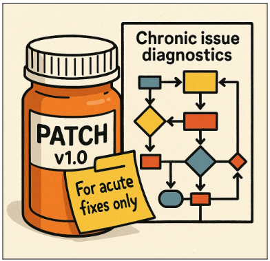
- Acute issues (e.g., BNPL fraud spike) → Treat first. Ship a quick rules-based patch to stop losses.
- Chronic issues (e.g., slow model drift) → Test more. Dig into root causes before retraining or adding complexity.
💡 Takeaway: The skill isn’t in always testing or always treating. It’s in diagnosing which response fits the situation — balancing speed with understanding — and ensuring today’s quick fix doesn’t become tomorrow’s chronic problem.
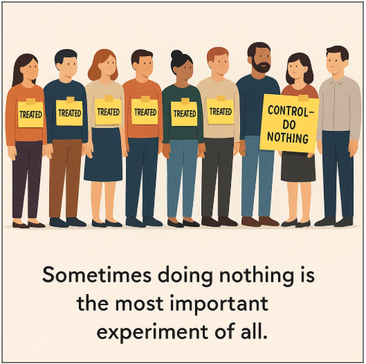
🧩 Control Sets – The Untreated Patients
In medicine, doctors sometimes leave a small group untreated to see if the new drug is truly helping — or if patients would have healed on their own.
In Simpl’s ML clinic, we do the same with control sets: they show us how the model behaves if we had done nothing — no promotions, no interventions, no fraud rules.
⚖️ Control Set Sizing
- Too large → we miss real opportunities and leave money on the table
- Too small → not enough statistical power to draw trustworthy conclusions
And because we deal with real money and real users, there’s another layer of responsibility. Control sets must be deterministically encrypted — so we can recreate the exact group later for analysis, and at the same time, ensure no one can reverse-engineer the system to game it.
💡 Takeaway: Control sets are the AI equivalent of blind clinical trials — a small, untreated sample that proves whether our “medicine” is truly working.
🩺 Differential Diagnosis — The Counterfactual Reasoning
Differential diagnosis means resisting the urge to guess, and instead systematically ruling out alternatives as new evidence arrives.
In this section, we’ll see it work in two separate examples:
- A medical case — a patient with fever, solved step by step using Bayesian reasoning.
- An ML case — a collapsing ROC-AUC curve, where we diagnose the root cause systematically.
🏥 Example 1 — Medical: The Fever Mystery
A patient walks in with fever, cough, and fatigue.
- Naïve approach: “It’s flu season → must be influenza → prescribe Tamiflu.”
- Differential diagnosis approach:
What if it’s pneumonia? What if it’s COVID-19? What if it’s early-stage leukemia?
Doctors don’t stop at first impressions. They run blood panels, chest X-rays, PCR tests. Each test eliminates some counterfactual worlds and updates the probabilities.
This is Bayesian reasoning in action — beliefs updated as evidence rolls in:
$$
P(H \mid E) = \frac{P(H) \cdot P(E \mid H)}{P(E)}
$$
Where:
- H = Hypothesis (possible diagnosis)
- E = Evidence (test results)
Step 1 — Define Hypotheses
We list our suspects: $H_1 = \text{Flu}, ; H_2 = \text{Pneumonia}, ; H_3 = \text{COVID-19}$
(Leukemia is possible in real life, but we’ll ignore it here to keep it simple.)
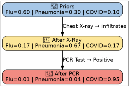
Step 2 — Priors (context before tests)
These are our priors—the initial beliefs before any new evidence arrives. $
P(H_1) = 0.6, \quad P(H_2) = 0.3, \quad P(H_3) = 0.1
$
It’s flu season, making flu the most likely cause (60%) ; pneumonia is less common; and COVID is even rarer.
Step 3 — Evidence #1: Chest X-Ray (shows infiltrates)
Now the patient gets a chest X-ray, and it shows lung infiltrates. We need to ask: How likely is this finding if each disease were true?
Likelihoods:
\[
P(E_{Xray}\mid Flu) = 0.1 \quad \text{(flu rarely causes infiltrates)} \\
P(E_{Xray}\mid Pneumonia) = 0.8 \quad \text{(pneumonia commonly shows infiltrates)} \\
P(E_{Xray}\mid COVID) = 0.6 \quad \text{(COVID sometimes looks like pneumonia)}
\]
Bayes update (numerators):
\[
\begin{align*}
\text{Flu} &: 0.6 \times 0.1 = 0.06 \\
\text{Pneumonia} &: 0.3 \times 0.8 = 0.24 \\
\text{COVID} &: 0.1 \times 0.6 = 0.06
\end{align*}
\]
Denominator:
\[
\begin{align*}
0.06 + 0.24 + 0.06 = 0.36
\end{align*}
\]
Posteriors (after X-ray):
\[
\begin{aligned}
P(\text{Flu} \mid E) &= \frac{0.06}{0.36} \approx 0.17 \\
P(\text{Pneumonia} \mid E) &= \frac{0.24}{0.36} \approx 0.67 \\
P(\text{COVID} \mid E) &= \frac{0.06}{0.36} \approx 0.17
\end{aligned}
\]
✅ After the X-ray, Pneumonia takes the lead (67%).
Step 4 — Evidence #2: COVID PCR Positive
PCR is highly specific and sensitive for COVID:
$$
P(E_{PCR}^+ \mid Flu)=0.01, \quad
P(E_{PCR}^+ \mid Pneumonia)=0.01, \quad
P(E_{PCR}^+ \mid COVID)=0.95
$$
Bayes update (numerators):
\begin{aligned}
Flu &: 0.17 \times 0.01 = 0.0017 \\
Pneumonia &: 0.67 \times 0.01 = 0.0067 \\
COVID &: 0.17 \times 0.95 = 0.1615
\end{aligned}
Denominator:
$
0.0017 + 0.0067 + 0.1615 = 0.1699
$
Posteriors:
\begin{aligned}
P(Flu\mid E) &= \tfrac{0.0017}{0.1699} \approx 0.01 \\
P(Pneumonia\mid E) &= \tfrac{0.0067}{0.1699} \approx 0.04 \\
P(COVID\mid E) &= \tfrac{0.1615}{0.1699} \approx 0.95
\end{aligned}
🔥 The PCR flips the story — COVID overwhelms the probability (95%).
⚖️ Final Lesson
At first, Flu appeared most likely (priors).
After the X-ray, Pneumonia seemed more probable.
Finally, the PCR made COVID the confirmed diagnosis.
Medical takeaway: Early priors favored flu; X-ray favored pneumonia; a decisive PCR flipped the story. In Bayesian reasoning, the “most likely” diagnosis is provisional—new evidence can completely reshape it.
🏥 Example 2 — 🤖 The Case of the Collapsing ROC–AUC 🫀
Your BNPL fraud detection model’s ROC-AUC suddenly nosedives in production or mid-training.
- Naïve approach: “Add more layers, train longer, and pray.”
- Differential diagnosis approach: Great data scientists don’t just throw treatments—they diagnose.
👉 A structured ML diagnosis has three steps:
Ⅰ. Pre-Diagnosis Essentials - pick the right metrics and evaluation setup.
Ⅱ. Diagnostic Tests - systematically check the model’s vitals, data, and pipeline.
Ⅲ. Treatment Options - apply targeted fixes based on the root cause.
Ⅰ • Pre-Diagnosis Essentials:
🎯 Choosing the right metric (thermometer vs. ECG)
If your dataset is balanced (≈50% fraud / 50% clean), ROC–AUC is fine — a broad health check across thresholds.
But when fraud is rare (say 10%), ROC–AUC is a blunt thermometer: it tells you something’s wrong but misses the nuance. What you really need is PR–AUC, your ECG, sensitive to those rare but critical events.
Let’s recall the vital signs:
$
Precision = \frac{TP}{TP+FP}, \quad
Recall = \frac{TP}{TP+FN}, \quad
F_1 = 2 \cdot \frac{Precision \cdot Recall}{Precision + Recall}
$
- Precision is the COVID rapid antigen test: if positive, it’s probably true.
- Recall is the COVID PCR: it tries not to miss anyone.
- F1-score balances both: don’t cry wolf, but don’t miss a wolf either.
And if business impact lies in the top 10% risk bucket, then you don’t care about the entire curve — only the sharp end:
$
Precision@q = \frac{1}{|S_q|}\sum_{i \in S_q} y_i, \quad
Recall@q = \frac{\sum_{i \in S_q} y_i}{\sum_{i=1}^N y_i}
$
where $S_q$ is your top $q%$ of scored users.
🧮 Train/Validation — Finding the right split
When you’re working with massive datasets (1M+ rows), the classic 80/20 split isn’t sacred. You can safely go as tight as 98/2 — just like in medicine, where despite having liters of blood, only a few drops are enough for reliable testing, as long as the sample represents the whole population and is large enough to be statistically sound.
🧭 Two OOTs — the second opinion
Most teams keep just one out-of-time set (OOT). That’s like trusting a single blood test for diagnosis.
But if you keep peeking at it during every retrain, you’re tuning to the test. The model starts memorizing quirks of that one future slice.
So you need two OOTs:
- OOT-A — the one you monitor regularly.
- OOT-B — a hidden “control set,” pulled only when you’re truly ready to validate.
If your model looks healthier on OOT-A but collapses on OOT-B, you’ve been overfitting to the wrong future.
Ⅱ • Diagnostic Tests
With the essentials set, it’s time for tests.
👀 Vital signs — is the model even alive?
First, check if the predictions are changing at all.
Flat outputs? The model is comatose.
Then move deeper: the gradients.
When training deep neural networks (esp. RNNs like LSTMs), gradients are propagated backwards through many layers or time steps.
The key object is the Jacobian of each layer’s transformation:
- $J_t =$ Jacobian (matrix of partial derivatives) at step $t$.
So when you backpropagate through $T$ layers/steps, the total gradient is: $\prod_{t=1}^T J_t$
This is a product of many Jacobians. Its norm (size) decides whether gradients survive, vanish, or explode.
- Exploding gradients are like a racing heartbeat — parameter updates blow up:
$
\Big|\prod_t J_t\Big| \gg 1 \quad \Rightarrow \quad \text{unstable swings}
$- If the product of Jacobians has a large norm, the gradient grows exponentially with depth/time.
- Result: parameter updates are huge and unstable.
- Analogy: a racing heartbeat — the model jumps around wildly instead of converging.
- Vanishing gradients are the faint pulse — no updates:
$
\Big|\prod_t J_t\Big| \ll 1 \quad \Rightarrow \quad \text{no learning}
$- If the product is very small, the gradient shrinks exponentially.
- By the time the signal reaches the early layers, it’s effectively zero.
- Result: weights don’t update → network can’t learn long-range dependencies.
- Analogy: a faint pulse — the model looks alive but isn’t learning.
These checks tell you whether the training loop is even alive.
🔎 Distribution scans — the CT scan of data
Now, check whether the world itself has changed.
- Data drift: Did new merchant types, customer behaviors, or transaction patterns sneak in - that the model never saw during training?
Run two-sample tests (e.g., KS statistic):
$
D_{KS} = \sup_x |F_{train}(x) - F_{prod}(x)|
$ - Feature expiration: Some features have a “shelf life.” For example, a holiday-specific indicator may become irrelevant or misleading after the holiday season.
- Leakage: the silent killer. It is like diagnosing diabetes by checking for insulin in the bag- perfect on paper, useless in practice. In data science, this happens when the model accidentally sees information that reveals the label. If you ever see ROC–AUC at 0.99, it’s probably not brilliance — it’s leakage masquerading as miracle performance.
⏮️ Historical backtesting — trust the patient’s records
Finally, compare today’s model with older checkpoints.
If a six-month-old model outperforms the new one, it’s not that yesterday’s model was a marvel — it’s that your new data or features are broken.
Ⅲ • Treatment Options
Once you’ve run the tests, then you prescribe.
🎛️ Stabilize the heartbeat
- Exploding gradients → Clip by Norm:
$
\nabla W \leftarrow \frac{\nabla W}{\max(1, |\nabla W|/\tau)}
$
Where:- ∇W = the gradient of weights (the update size).
- ∣∣∇W∣∣ = the norm (magnitude) of the gradient vector.
- τ = the threshold (clip value you set).
👉 What it does:
- If the gradient norm is smaller than τ, nothing changes.
- If the gradient norm is larger than τ, the whole gradient vector is rescaled down so that its size is capped at τ.
Lowering the learning rate, adding in layer normalisation and monitoring the update magnitudes can also help keep training stable.
⚖️ Analogy: Imagine you’re pouring water into a cup. If you pour too fast (exploding gradients), water spills everywhere. Gradient clipping is like putting a lid on the cup — no matter how hard you pour, the flow that gets in is capped.
- Vanishing gradients → switch to LSTMs / GRUs, add residual connections, use better initialization strategies (He/Xavier). Keep signals alive.
⚖️ Dosing bias vs variance
- Underfitting (high bias): When a model suffers from underfitting, it’s too simple to capture meaningful patterns. You’ll notice this when both training and validation accuracy are low. Think of it like giving a patient too weak a dose of antibiotics: the infection keeps spreading because the treatment is insufficient. The fix is to ease off on regularization or give the model more capacity — deeper networks, richer features, or simply more training.
- Overfitting (high variance): On the other hand, overfitting happens when the model memorizes the training data but fails on new data. Here, training accuracy looks great, but validation/test accuracy collapses. This is like prescribing too much medicine: yes, it wipes out the infection, but it also harms healthy cells, leaving the patient fragile in the real world. To treat this, you add dropout, strengthen regularization, or stop training early — essentially making the model less obsessed with memorization and more focused on general patterns.
- The art of data science here is balancing the dose: Too little treatment leads to underfitting; too much treatment causes overfitting. Just the right balance cures the patient — or in ML terms, delivers a model that generalizes well.
🧼 Data hygiene — remove the infection
- Drift? Retrain faster, shorten feature windows.
- Feature expiration? Retire or re-encode.
- Leakage? Rewrite features with strict cutoffs.
🛠️ Calibrate and threshold wisely
Remember: the business doesn’t care about ROC–AUC or PR-AUC, it cares about decisions. Set thresholds at the top segment, calibrate probabilities, and monitor Brier scores. When your model says “25% fraud risk,” the business expects that to line up with reality — not just be a model’s guess. That’s what the Brier score keeps you honest about.
$$
Brier = \frac{1}{N}\sum_{i=1}^N(\hat p_i - y_i)^2
$$
💡 Takeaway: Don’t just throw layers and compute at the problem. Run diagnostics first, then treat the actual root cause. This saves time, prevents false confidence, and makes your data science model far more reliable in production.

🏁 Conclusion: Think Like a Diagnostician
At Simpl, we treat our ML pipeline like a clinic:
- Symptoms → anomalies, alerts, user churn
- Tests → experiments, shadow deployments, ablations
- Treatments → feature rollouts, retrains, UX changes
- Relapse → drift, bias recurrence
Great data scientists aren’t just model builders — they’re diagnosticians. They embrace co-morbid causes, treat with humility, and always ask:
“Why is this working — and would it still work without this?”
Whether it’s curing fraud spikes, tuning LSTMs, or running growth experiments, our approach at Simpl is clear: “Understanding the model beats iterating in the dark”
💡 And remember… It’s never lupus.